Beyond the Average: Understanding Variance, Standard Deviation, and Coefficient of Variation 📊

Welcome, data enthusiasts! If you’ve ever looked at a dataset and thought, “The average is 50, but what does that really tell me?” then you’ve asked the right question. The mean, or average, is a great starting point, but it only tells part of the story. It hides the drama, the spread, and the consistency within your data.

In statistics and data analysis, three fundamental measures help us understand the spread or dispersion of data: Variance, Standard Deviation, and Coefficient of Variation (CV). While averages (like the mean) tell us the “central” value of data, these measures reveal how much the data fluctuates around that average.

To get the full picture, we need to understand variability. Today, we’re diving into three fundamental pillars of statistics that measure exactly that: Variance, Standard Deviation, and the Coefficient of Variation.

Why Just the Average Isn’t Enough

Let’s start with a simple example. Imagine we have test scores out of 100 for two different classes, both with an average score of 70.

Class A Scores: 68, 69, 70, 71, 72
Class B Scores: 50, 60, 70, 80, 90

Both have a mean of 70. But are these classes performing similarly? Absolutely not! Class A is incredibly consistent, with everyone scoring very close to the average. Class B is all over the place, with both high achievers and those who struggled.

This “spread” or “dispersion” is what Variance and Standard Deviation help us quantify.

🔹 1. Variance: The Average of Squared Differences

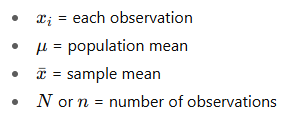
Variance (σ² for a population, s² for a sample) is the foundation. It measures how far each data point in a set is from the mean. The calculation might look a bit intimidating at first, but the concept is straightforward. Variance is the average of the squared differences between each data point and the mean. It measures how spread out the data points are.

How to Calculate Variance:

Find the mean (the average) of the dataset.
Find the difference between each data point and the mean.
Square each of these differences (this makes all values positive and emphasizes larger differences).
Find the average of these squared differences.

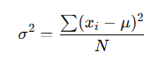
Formula (Population Variance):

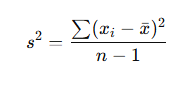
Formula (Sample Variance):

Why square the differences? If we just added up the raw differences (e.g., (68-70) + (69-70)…), the positive and negative values would cancel each other out, giving us zero—which isn’t helpful. Squaring solves this problem.

Let’s calculate the variance for our two classes:

Class A (Mean = 70)

Score	Difference from Mean (Score – 70)	Squared Difference
68	-2	4
69	-1	1
70	0	0
71	1	1
72	2	4
Sum of Squared Differences		10

Variance for Class A = 10 / 5 (number of students) = 2

Class B (Mean = 70)

Score	Difference from Mean (Score – 70)	Squared Difference
50	-20	400
60	-10	100
70	0	0
80	10	100
90	20	400
Sum of Squared Differences		1000

Variance for Class B = 1000 / 5 = 200

Interpretation: Class A has a variance of 2, and Class B has a variance of 200. The much larger variance for Class B confirms what we saw visually—its scores are far more spread out.

The Catch with Variance: The units are squared. Since our data was “points,” the variance is in “points².” This isn’t very intuitive to interpret in the real world. That’s where Standard Deviation comes in.

🔹 2. Standard Deviation: The King of Spread

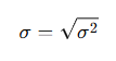
Standard Deviation (σ for a population, s for a sample) is simply the square root of the variance. It’s the most common and useful measure of spread.

By taking the square root, we bring the units back to their original form (e.g., just “points” instead of “points²”), making it instantly understandable.

How to Calculate Standard Deviation:

Calculate the variance.
Take the square root of the variance.

It’s that simple!

Formula:

Let’s calculate it for our classes:

Class A Standard Deviation: √2 ≈ 1.41 points
Class B Standard Deviation: √200 ≈ 14.14 points

Interpretation: You can now say, “The typical score in Class A is within 1.41 points of the average (70),” indicating high consistency. For Class B, “The typical score is within about 14 points of the average,” indicating much higher variability.

Standard deviation gives you a direct, intuitive sense of the “typical” distance from the average. It’s used everywhere—from finance (measuring investment risk) to manufacturing (controlling product quality).

🔹 3. Coefficient of Variation: The Relative Comparison

Now for a trickier question: How do you compare the spread of two datasets that are measured in different units or have very different means?

For example:

Dataset 1: The height of oak trees (in meters, mean = 20m, SD = 5m)
Dataset 2: The weight of oak trees (in kilograms, mean = 500kg, SD = 100kg)

Which is more variable, the height or the weight? We can’t compare 5 meters to 100 kilograms. This is the problem the Coefficient of Variation (CV) solves.

The CV is a standardized, unit-less measure of dispersion. It is defined as:

Formula:

Coefficient of Variation (CV) = (Standard Deviation / Mean) × 100%

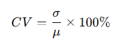
It expresses the standard deviation as a percentage of the mean, allowing for a pure relative comparison.

Let’s calculate it for our tree example:

Height CV: (5 / 20) × 100% = 25%
Weight CV: (100 / 500) × 100% = 20%

Interpretation: The height of the trees has a coefficient of variation of 25%, while the weight has a CV of 20%. This means that relative to their respective averages, the heights are more variable than the weights.

Another Example: Comparing Investment Risk
Imagine two potential investments:

Investment X: Mean return = 8%, Standard Deviation = 5%
Investment Y: Mean return = 4%, Standard Deviation = 3%

Which is riskier (more volatile) relative to its expected return?

CV for X: (5 / 8) × 100% = 62.5%
CV for Y: (3 / 4) × 100% = 75%

Even though Investment X has a higher absolute standard deviation, Investment Y has a higher CV. This means its risk is higher relative to its smaller expected return. An investor might see Investment Y as a less efficient choice.

🔹 Key Differences

Measure	What it Shows	Units	Useful For
Variance	Average squared deviation from mean	Squared units	Mathematical/statistical models
Standard Deviation	Typical distance from mean	Same as data	Easy interpretation
Coefficient of Variation	Relative spread in %	Dimensionless	Comparing across datasets

🔹 Real-Life Applications

Finance – Standard deviation measures risk in stock returns. CV compares volatility across different stocks.
Manufacturing – Low standard deviation indicates consistent product quality.
Education – Variance in exam scores helps teachers identify uniformity or diversity in student performance.
Healthcare – CV is used to compare variability in patient health metrics across populations.

Summary & When to Use What

Measure	Symbol (Sample)	What it Does	Best Used For
Variance	s²	Measures the average squared deviation from the mean.	The foundational calculation. Less interpretable due to squared units.
Standard Deviation	s	Measures the typical deviation from the mean.	Understanding spread in the context of the data’s units. The go-to measure for variability. (e.g., “The average height is 175cm, with a standard deviation of 10cm.”)
Coefficient of Variation	CV	Measures the relative variability as a percentage.	Comparing the spread of datasets with different units or vastly different means. (e.g., comparing stock volatility to commodity volatility.)

✅ Key Takeaway

Don’t let your data analysis stop at the average. To truly understand what your data is telling you, you must ask about its spread.

Use Variance as the calculation behind the scenes.
Use Standard Deviation to understand variability in context.
Use the Coefficient of Variation to make apples-to-oranges comparisons between different datasets.

Variance → squared measure of spread.

Standard Deviation → average deviation, easier to interpret.

Coefficient of Variation → relative measure (useful for comparison).

By mastering these three concepts, you’ll move from simply describing the center of your data to fully capturing its story—variability, consistency, and all.

👉 Now go forth and analyze with confidence

📚 Further Reading

If you’d like to explore more about measures of dispersion and their applications, here are some useful resources

Statistics for Business and Economics by Paul Newbold, William L. Carlson, and Betty Thorne – A comprehensive book with real-world applications.
The Art of Statistics by David Spiegelhalter – A beginner-friendly guide to understanding statistics in daily life.
Business Statistics by Ken Black – Covers dispersion measures with practical examples and exercises.