📊 Normal Distribution: Concepts, Properties, Applications & Examples

1. Introduction

In statistics, one of the most important and widely used concepts is the normal distribution, also known as the Gaussian distribution. It plays a central role in data analysis, probability theory, and inferential statistics because many real-world phenomena approximately follow this distribution.

From students’ test scores to measurement errors and biological traits like height and weight, the normal distribution provides a powerful framework to understand variability and uncertainty.

2. What is Normal Distribution?

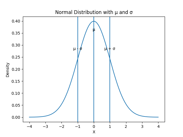
A normal distribution is a continuous probability distribution that is symmetric about its mean. It is characterized by a bell-shaped curve where:

Most observations cluster around the central peak (mean)
Probabilities decrease as we move away from the mean
The distribution is perfectly symmetrical

Mathematically, it is defined by two parameters:

Mean (μ) → Center of the distribution
Standard Deviation (σ) → Spread or dispersion of the data

3. Mathematical Representation

The probability density function (PDF) of a normal distribution is:

Where:

x = random variable
μ = mean
σ = standard deviation

This formula defines the shape of the bell curve.

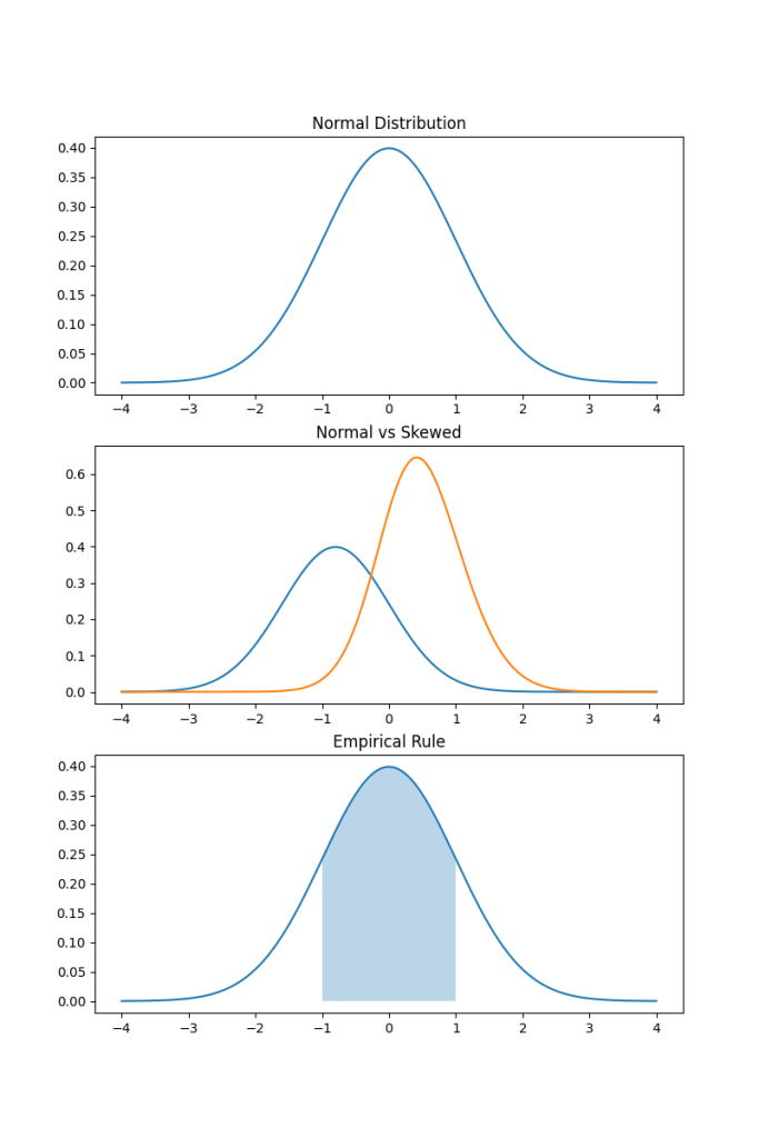
4. Key Properties of Normal Distribution

✔️ Symmetry

The distribution is symmetric around the mean.
Mean = Median = Mode

✔️ Bell-Shaped Curve

Highest point at the mean
Tails extend infinitely in both directions

✔️ Total Area = 1

The total probability under the curve equals 1

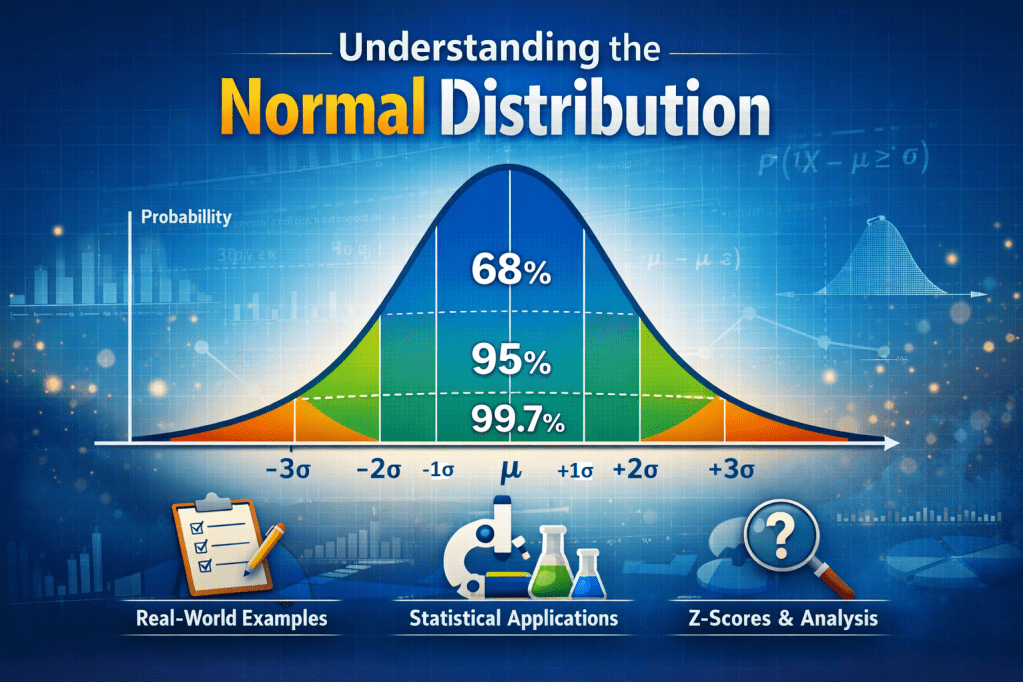
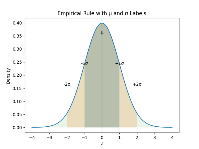
✔️ Empirical Rule (68-95-99.7 Rule)

This means:

68% of data lies within ±1σ
95% within ±2σ
99.7% within ±3σ

5. Standard Normal Distribution (Z-Distribution)

When a normal distribution is standardized, it becomes a standard normal distribution with:

Mean = 0
Standard deviation = 1

The transformation is:

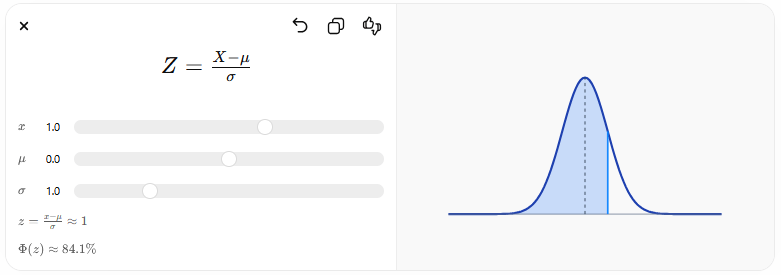
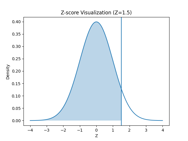
This conversion allows us to use Z-tables to find probabilities.

6. Real-World Examples

📌 Example 1: Students’ Exam Scores

Suppose exam scores are normally distributed:

Mean (μ) = 70
Standard deviation (σ) = 10
About 68% of students score between 60 and 80
About 95% score between 50 and 90

📌 Example 2: Human Height

Heights of adult males in a population often follow a normal distribution:

Mean = 170 cm
Standard deviation = 7 cm

Most individuals fall within:

163–177 cm (±1σ)

📌 Example 3: Measurement Errors

In scientific experiments:

Small errors occur frequently
Large errors are rare
This pattern forms a normal distribution.

7. Applications of Normal Distribution

🎓 1. Education & Testing

Grading systems
Standardized tests (e.g., percentile ranks)

💼 2. Business & Management

Demand forecasting
Quality control (Six Sigma)

🌾 3. Agriculture Research

Crop yield variability
Experimental error analysis

🧪 4. Scientific Research

Sampling distributions
Hypothesis testing

💰 5. Finance

Risk modeling
Asset return analysis (approximation)

8. Why is Normal Distribution Important?

🔹 Central Limit Theorem (CLT)

One of the key reasons for its importance is the Central Limit Theorem, which states:

The sampling distribution of the mean tends to be normal, regardless of the population distribution (for large sample sizes).

This makes the normal distribution foundational for:

Statistical inference
Confidence intervals
Hypothesis testing

9. Limitations of Normal Distribution

Despite its usefulness, it has some limitations:

Not suitable for skewed data
Cannot model extreme outliers effectively
Assumes infinite range (−∞ to +∞)
Real-world data may have fat tails (e.g., financial crashes)

10. Visual Interpretation (Conceptual)

A normal curve:

Peaks at the mean
Tapers symmetrically
Has inflection points at ±1σ

11. Conclusion

The normal distribution is a cornerstone of statistics due to its simplicity, mathematical elegance, and wide applicability. Whether in agriculture, management, or scientific research, understanding this distribution helps in making informed decisions based on data.

Mastering normal distribution also opens the door to advanced statistical techniques such as regression analysis, hypothesis testing, and machine learning models.

📚 References

Montgomery, D. C., & Runger, G. C. (2014). Applied Statistics and Probability for Engineers
Gupta, S. C., & Kapoor, V. K. (2020). Fundamentals of Mathematical Statistics
Spiegel, M. R. (2009). Schaum’s Outline of Statistics
Walpole, R. E. et al. (2012). Probability and Statistics for Engineers and Scientists
Khan Academy – Normal Distribution Tutorials
NIST/SEMATECH e-Handbook of Statistical Methods