🌟 Introduction

In business, supply chains, finance, manufacturing, agriculture, transport, and even daily planning, we constantly face situations where resources are limited. Linear Programming (LP) is one of the most powerful mathematical tools to allocate scarce resources optimally.

From choosing the best product mix, minimizing transportation costs, or optimizing crop planning, LP turns complex decisions into solvable mathematical models.

---

🔍 What is Linear Programming?

Linear Programming (LP) is a mathematical optimization technique used to determine the best possible outcome under a set of linear constraints.

In simple terms:

Linear Programming helps you maximize profit or minimize cost while satisfying certain resource limitations.

---

🎯 Components of a Linear Programming Model

Any LP model consists of four key components:

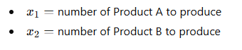
1️⃣ Decision Variables

These represent the choices to be made.
Example:

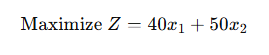
2️⃣ Objective Function

This is what you want to maximize (profit) or minimize (cost).

Example:

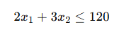
3️⃣ Constraints

These represent the resource limitations.

Examples:

• Machine hours
• Budget limits
• Labor
• Raw materials

These constraints must be linear, e.g.,

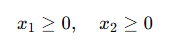
4️⃣ Non-negativity Constraints

Since negative production is impossible:

---

🧱 Mathematical Structure of an LP Model

---

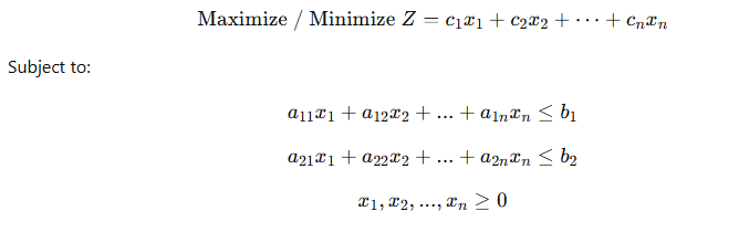
🧮 Solved Example 1: Product Mix Optimization (Graphical Method)

A company produces two products, A and B.

Resource	Product A	Product B	Availability
Machine Hours	2	3	120
Labor Hours	3	2	100

Profit:

• Product A: ₹40
• Product B: ₹50

---

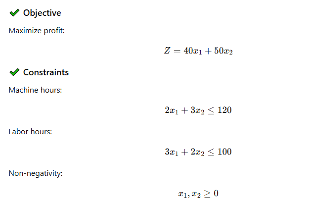
Step 1: Convert constraints to lines

---

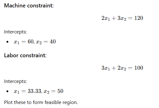
Step 2: Identify corner points

The feasible region corner points are:

1. (0, 0)
2. (0, 40)
3. Intersection of both constraints
4. (33.33, 0)

---

Step 3: Solve intersection point

---

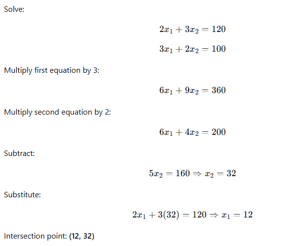
Step 4: Evaluate objective function

Point	Profit Z
(0, 0)	0
(0, 40)	2000
(33.33, 0)	1333.2
(12, 32)	40×12 + 50×32 = 800 + 1600 = 2400

---

⭐ Optimal Solution

Produce:

• 12 units of A
• 32 units of B

Maximum Profit = ₹2400

---

🧮 Solved Example 2: Diet Optimization Problem

A person wants to meet nutritional needs at minimum cost.

Food A and B provide nutrients as:

Nutrient	Food A	Food B	Requirement
Protein	4	2	≥ 12
Carbs	2	4	≥ 12
Cost	₹6	₹8	Minimize

✔ Decision variables

x = units of Food A
y = units of Food B

---

---

Solve intersections

---

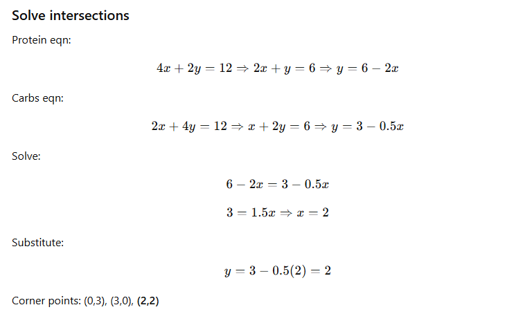
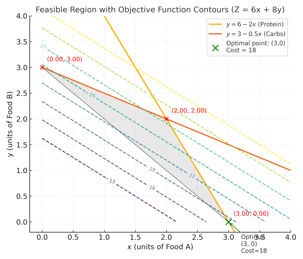
Evaluate cost:

• (3,0): 6×3 = 18
• (0,3): 8×3 = 24
• (2,2): 6×2 + 8×2 = 28

Minimum is actually 18 at (3,0).

⭐ Optimal Solution

Eat:

• 3 units of Food A
• 0 units of Food B

Minimum cost = ₹18

---

📊 Applications of Linear Programming

Industry	LP Application
Manufacturing	Product mix, job scheduling
Logistics	Transportation & routing
Agriculture	Crop planning, fertilizer allocation
Energy	Grid optimization
Finance	Portfolio optimization
Marketing	Budget allocation
Healthcare	Staff scheduling, resource planning

---

🔧 Solving LP in Python (PuLP)

---

🧾 Final Takeaways

✔ LP is one of the most widely used optimization tools.
✔ Helps allocate limited resources optimally.
✔ Works best when relationships are linear.
✔ Solvable using both graphical method (2 variables) and Simplex Method (many variables).

---

📚 Further Reading

• Fred Hillier & Gerald Lieberman – Introduction to Operations Research
• Bazaraa, Jarvis & Sherali – Linear Programming and Network Flows
• Winston – Operations Research: Applications and Algorithms

---