Statistics isn’t just about averages — it’s also about testing relationships between variables. One of the most commonly used statistical tools for this purpose is the Chi-Square (χ²) Test.

Whether you’re analyzing survey data, market preferences, or categorical outcomes, the Chi-Square test helps you determine if an observed difference or relationship is real or just due to chance.

---

🔹 What is a Chi-Square Test?

Welcome back, data enthusiasts! So far, we’ve explored how to measure spread in numerical data. But what happens when your data isn’t numbers, but categories? For instance, does gender influence political party preference? Is there a link between a marketing campaign and a customer’s purchase decision?

To answer these questions, we need a different tool—one designed for counts and categories. Enter the Chi-Square Test (pronounced “Kai-Square”).

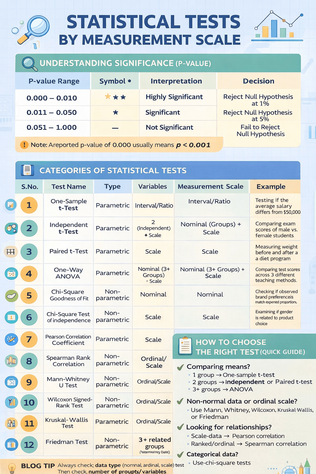
The Chi-Square Test (χ²) is a non-parametric test used to determine whether there is a significant association between categorical variables or whether the observed frequencies differ from expected frequencies. It compares the actual data you observed with the data you would expect if there were no relationship between the variables.

At its heart, the Chi-Square test checks if there’s a significant relationship between two categorical variables or if the distribution of one categorical variable fits a specific expectation. It does this by comparing what we observe in the real world to what we would expect to see if there were no relationship (i.e., if they were independent).

The Core Idea: Observed vs. Expected

The entire test hinges on a simple comparison:

• Observed Frequency (O): The actual counts you recorded in your data.
• Expected Frequency (E): The counts you would expect if there was no relationship between the variables.

If the differences between Observed (O) and Expected (E) counts are large, it suggests a relationship exists. If the differences are small, it’s likely due to random chance.

---

🔹 Formula

Where:

• (O) = Observed frequency
• (E) = Expected frequency

If the calculated χ² value is greater than the critical value (from the Chi-square table for given degrees of freedom and significance level), we reject the null hypothesis.

---

🔹 Types of Chi-Square Tests

Type	Purpose	Example
1. Chi-Square Goodness of Fit Test	Tests if a sample data matches a population distribution.	Checking if dice is fair.
2. Chi-Square Test of Independence	Tests if two categorical variables are related.	Checking if gender and product preference are related.
3. Chi-Square Test for Homogeneity	Tests if distributions are the same across multiple populations.	Comparing age groups and their choice of a streaming service.

---

🔹 1. Chi-Square Goodness of Fit Test Example

🧮 Problems:

Example 1

A die is rolled 60 times, and the results are:

Face	1	2	3	4	5	6
Observed (O)	8	9	10	12	11	10

Is the die fair at 5% significance level?

✅ Step 1: Hypotheses

• H₀: The die is fair (all faces have equal probability).
• H₁: The die is not fair.

✅ Step 2: Expected Frequency

If the die is fair:

✅ Step 3: Compute χ²

Face	O	E	(O−E)²/E
1	8	10	0.4
2	9	10	0.1
3	10	10	0.0
4	12	10	0.4
5	11	10	0.1
6	10	10	0.0

χ2 = 0.4 + 0.1 + 0.0 + 0.4 + 0.1 + 0.0 = 1.0

✅ Step 4: Decision

Degrees of freedom (df) = 6 – 1 = 5
Critical χ² value at 5% = 11.07

Since 1.0 < 11.07,
✅ Fail to reject H₀. The die is fair.

Example 2

The Colored Candy Problem

A candy company claims that its “Rainbow Mix” is distributed as follows: 30% Red, 20% Yellow, 25% Green, and 25% Blue. You buy a large bag containing 400 candies to test their claim. Your observed counts are:

• Red: 130
• Yellow: 80
• Green: 90
• Blue: 100

Does your sample support the company’s claim?

Step 1: State the Hypotheses

• Null Hypothesis (H₀): The distribution of candy colors matches the company’s claim.
• Alternative Hypothesis (H₁): The distribution of candy colors does not match the claim.

Step 2: Calculate the Expected Frequencies (E)

This is easier. We simply apply the claimed percentages to our total sample size.

• Expected Red: 30% of 400 = 120
• Expected Yellow: 20% of 400 = 80
• Expected Green: 25% of 400 = 100
• Expected Blue: 25% of 400 = 100

Step 3: Calculate the Chi-Square Statistic (χ²)

We use the same formula: χ² = Σ [ (O – E)² / E ]

Color	O	E	O – E	(O – E)²	(O – E)² / E
Red	130	120	10	100	0.833
Yellow	80	80	0	0	0.000
Green	90	100	-10	100	1.000
Blue	100	100	0	0	0.000
Total (χ²)					1.833

Our calculated Chi-Square test statistic is χ² = 1.833.

Step 4: Find the Critical Value and Make a Decision

• Significance Level (α): 0.05
• Degrees of Freedom (df): For goodness of fit, df = (number of categories – 1). We have 4 colors, so df = 3.

The critical value from the Chi-Square table for df=3 and α=0.05 is 7.815.

Decision:

• Our χ² (1.833) < Critical Value (7.815)

Step 5: Conclusion

We fail to reject the null hypothesis. There is not enough evidence to say that the candy color distribution is different from what the company claims. Your bag’s contents are consistent with their advertised proportions.

---

🔹 2. Chi-Square Test of Independence Example

🧮 Problem:

Example 1

A company wants to know if gender and product preference are related.

Gender	Product A	Product B	Total
Male	30	10	40
Female	20	20	40
Total	50	30	80

✅ Step 1: Hypotheses

• H₀: Gender and product preference are independent.
• H₁: They are related.

✅ Step 2: Compute Expected Frequencies

Cell	Formula	E
Male, A	(40×50)/80	25
Male, B	(40×30)/80	15
Female, A	(40×50)/80	25
Female, B	(40×30)/80	15

✅ Step 3: Compute χ²

Cell	O	E	(O−E)²/E
Male, A	30	25	1.0
Male, B	10	15	1.67
Female, A	20	25	1.0
Female, B	20	15	1.67

✅ Step 4: Decision

df = (2−1)(2−1) = 1
Critical χ² value at 5% = 3.84

Since 5.34 > 3.84,
❌ Reject H₀.
✅ Gender and product preference are related.

Example 2

Ice Cream Flavor & Gender

A local ice cream shop wants to know if gender is independent of favorite ice cream flavor. They survey 200 customers and get the following results:

Observed Frequencies (O)

Flavor	Men	Women	Row Total
Chocolate	30	40	70
Vanilla	20	30	50
Strawberry	25	55	80
Column Total	75	125	200 (Grand Total)

At a glance, it seems women might prefer Strawberry more. But is this a real pattern or just a random fluke? The Chi-Square test can tell us.

Step 1: State the Hypotheses

• Null Hypothesis (H₀): There is no relationship between gender and ice cream preference. The variables are independent.
• Alternative Hypothesis (H₁): There is a relationship between gender and ice cream preference.

Step 2: Calculate the Expected Frequencies (E)

The expected count for each cell is calculated as:
E = (Row Total × Column Total) / Grand Total

This is the core formula! It represents the count we’d expect if flavor preference was distributed proportionally across genders.

• Expected Men who like Chocolate: (70 × 75) / 200 = 52.5 / 200 = 26.25
• Expected Women who like Chocolate: (70 × 125) / 200 = 8750 / 200 = 43.75
• Expected Men who like Vanilla: (50 × 75) / 200 = 3750 / 200 = 18.75
• Expected Women who like Vanilla: (50 × 125) / 200 = 6250 / 200 = 31.25
• Expected Men who like Strawberry: (80 × 75) / 200 = 6000 / 200 = 30
• Expected Women who like Strawberry: (80 × 125) / 200 = 10000 / 200 = 50

Expected Frequencies (E) Table

Flavor	Men	Women
Chocolate	26.25	43.75
Vanilla	18.75	31.25
Strawberry	30.00	50.00

Step 3: Calculate the Chi-Square Statistic (χ²)

The formula for the test statistic is:
χ² = Σ [ (O – E)² / E ]

Where Σ means “sum of” and we calculate (O-E)²/E for every single cell in the table.

Let’s calculate it for each cell:

Cell	O	E	O – E	(O – E)²	(O – E)² / E
Men, Chocolate	30	26.25	3.75	14.06	0.536
Women, Chocolate	40	43.75	-3.75	14.06	0.321
Men, Vanilla	20	18.75	1.25	1.56	0.083
Women, Vanilla	30	31.25	-1.25	1.56	0.050
Men, Strawberry	25	30.00	-5.00	25.00	0.833
Women, Strawberry	55	50.00	5.00	25.00	0.500
Total (χ²)					2.323

Our calculated Chi-Square test statistic is χ² = 2.323.

Step 4: Find the Critical Value and Make a Decision

We need to compare our statistic to a critical value from a Chi-Square distribution table. To do this, we need:

• Significance Level (α): Typically 0.05 (5%).
• Degrees of Freedom (df): For a test of independence, df = (number of rows – 1) × (number of columns – 1). In our case, (3-1) × (2-1) = 2.

Looking up the critical value for df=2 and α=0.05, we find it is 5.991.

Decision Rule: If our χ² statistic is greater than the critical value, we reject the null hypothesis.

• Our χ² (2.323) < Critical Value (5.991)

Step 5: Conclusion

We fail to reject the null hypothesis. There is not enough evidence to conclude a significant relationship between gender and ice cream preference at the 5% significance level. The differences we observed in our sample are likely due to random chance.

---

🔹 When to Use the Chi-Square Test

Situation	Use
Checking fairness of dice, coin, or survey distribution	Goodness of Fit
Testing relationship between variables (like age and satisfaction)	Test of Independence
Comparing multiple populations	Test for Homogeneity

---

🔹 Assumptions of the Chi-Square Test

Before you run off to chi-square everything, remember these crucial rules:

• Data should be in frequency (count) form, not percentages.
• Categorical Data: Your data must be in categories (counts or frequencies). Categories should be mutually exclusive.
• Independence: Observations must be independent of each other.
• Sample Size: The expected frequency (E) for any cell should not be less than 5. (Some relax this to 80% of cells should have E > 5). If this assumption is violated, the test may not be valid.

---

🔹 Interpretation Guidelines

χ² value	p-value	Interpretation
Small	> 0.05	No significant difference (accept H₀)
Large	< 0.05	Significant difference (reject H₀)

---

🧠 Quick Summary

• Chi-Square (χ²) compares observed vs expected frequencies.
• Used for categorical (nominal) data.
• Two main tests: Goodness of Fit and Independence.
• Higher χ² → stronger evidence against null hypothesis.

The Chi-Square test is a powerful, fundamental tool for unlocking stories hidden in categorical data.

• Use the Test of Independence to explore relationships between two variables (e.g., “Is smoking linked to lung cancer?”).
• Use the Goodness of Fit Test to see if your data matches a theoretical distribution (e.g., “Does the ratio of plant phenotypes match Mendelian genetics?”).

By comparing what you see to what you’d expect by chance, you can move beyond guesswork and make robust, data-driven conclusions about the world of categories.

---

📚 Further Reading

• Khan Academy – Chi-Square Tests
• Investopedia – Chi-Square Test
• Statistics for Business and Economics by Newbold et al.

---