🌟 Introduction

In data analysis and inferential statistics, we often want to test hypotheses about population means — for example:

Do two groups differ significantly in their average income?
Does a new fertilizer increase crop yield compared to the previous one?
Are the exam scores of two classes statistically different?

To answer such questions, we use statistical hypothesis testing, and two of the most commonly used tools are the t-test and z-test.

Though both serve similar purposes — testing differences in means — they differ in sample size, data variance knowledge, and underlying assumptions.

🎯 What Are Hypothesis Tests?

Hypothesis testing helps us make decisions about a population based on sample data.

We start with:

Null Hypothesis (H₀): No difference or effect exists.
Alternative Hypothesis (H₁): There is a significant difference or effect.

We then calculate a test statistic (like t or z) to determine whether to reject H₀.

⚖️ Difference Between t-Test and Z-Test

Feature	t-Test	Z-Test
Population standard deviation (σ)	Unknown	Known
Sample size (n)	Small (n < 30)	Large (n ≥ 30)
Distribution used	t-distribution	Normal (z) distribution
Use case	Compare means when σ unknown	Compare means when σ known
Example	Comparing two classroom averages	Comparing a sample mean to population mean

💡 Tip: When in doubt and σ is unknown (which is common in real life), use the t-test.

🧮 The Formulas

Z-Test Formula:

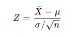
Where:

x̄: Your sample mean
μ: The known population mean
σ: The known population standard deviation
n: Your sample size

t-Test Formula:

Where:

s = sample standard deviation (since σ is unknown)

📊 Types of t-Tests

Type	Used When	Example
One-sample t-test	Comparing a sample mean to a known population mean	Is the average yield from a new crop variety = 40 kg/acre?
Independent two-sample t-test	Comparing means of two independent groups	Do male and female students differ in average scores?
Paired sample t-test	Comparing two related groups (before-after)	Did training improve employee productivity?

The t-Test

In the real world, you rarely know the population standard deviation (σ). You only have your sample to work with. The t-test is the modern solution to this problem, using the sample standard deviation (s) instead.

When to Use a t-test:

Your sample size is small (typically n < 30).
You do not know the population standard deviation (σ).
Your data is (approximately) normally distributed.

The t-test accounts for the extra uncertainty introduced by estimating σ from the sample. This makes its distribution (the t-distribution) slightly wider and flatter than the normal Z-distribution.

The t-Test Statistic Formula (One-Sample):
t = (x̄ - μ) / (s / √n)

s: The sample standard deviation

Solved Example: The New Drug Trial

A pharmaceutical company claims its new drug reduces cholesterol by an average of 30 points (the known population mean for the old drug). A small clinical trial with 15 patients uses the new drug. The sample mean reduction is 35 points with a sample standard deviation of 8 points. Test if the new drug is more effective at α = 0.05.

Step 1: State the Hypotheses

H₀: The new drug is not more effective. μ = 30 points.
H₁: The new drug is more effective. μ > 30 points. (One-tailed test)

Step 2: Calculate the t-Test Statistic
We have:

x̄ = 35 points
μ = 30 points
s = 8 points
n = 15

t = (35 - 30) / (8 / √15) = (5) / (8 / 3.873) = 5 / 2.066 ≈ 2.420

Step 3: Find the Critical Value and Make a Decision
We need the critical value from the t-distribution table.

Degrees of Freedom (df): df = n - 1 = 15 - 1 = 14
Significance Level (α): 0.05 for a one-tailed test.

The critical t-value for df=14 and α=0.05 (one-tailed) is 1.761.

Decision Rule: If our t-statistic is greater than the critical value, we reject the null hypothesis.

Our t (2.420) > Critical t (1.761)

Step 4: Conclusion
We reject the null hypothesis. There is sufficient evidence to conclude that the new drug leads to a greater average reduction in cholesterol than the old drug.

📘 Example 1: One-Sample Z-Test

Scenario:
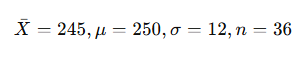
A tea factory claims that the average weight of tea packets is 250g.
A consumer group randomly samples 36 packets and finds the mean weight = 245g, with σ = 12g.
Test at 5% significance if the claim is valid.

Step 1:
H₀: μ = 250
H₁: μ ≠ 250

Step 2:
Given:

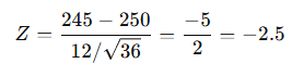
Step 3: Compute Z-statistic

Step 4:
At α = 0.05 (two-tailed), critical Z = ±1.96

Step 5:
Since |−2.5| > 1.96 → Reject H₀

✅ Conclusion: The mean weight differs significantly from 250g; the claim is not valid.

📗 Example 2: One-Sample t-Test

Scenario:
A farmer believes the average yield of his farm is 60 kg per acre.
From a sample of 16 plots, the mean yield is 58 kg, and the sample standard deviation is 4 kg.
Test the farmer’s claim at 5% significance.

Step 1:
H₀: μ = 60
H₁: μ ≠ 60

Step 2:
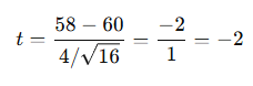
Given:
x̄=58, μ=60, s=4, n=16

Step 3: Compute t-statistic

Step 4:
Degrees of freedom (df) = n − 1 = 15
From t-table at α = 0.05, two-tailed, critical t = ±2.131

Step 5:
|−2| < 2.131 → Fail to reject H₀

✅ Conclusion: The farmer’s claim is valid; there’s no significant difference from 60 kg/acre.

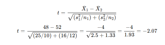
📘 Example 3: Independent Two-Sample t-Test

Scenario:
You want to know if two fertilizers (A and B) yield different average outputs.

Fertilizer	Mean Yield (kg/acre)	Sample Size	Std. Dev.
A	48	10	5
B	52	12	4

Test at 5% significance.

Step 1:
H₀: μ₁ = μ₂
H₁: μ₁ ≠ μ₂

Step 2:

Step 3:
df ≈ n₁ + n₂ − 2 = 20
Critical t = ±2.086

Step 4:
|−2.07| < 2.086 → Fail to reject H₀

✅ Conclusion: There is no significant difference between Fertilizer A and B yields.

📘 Example 3: Paired Sample t-Test

Scenario: A coach wants to know whether a 4-week training program improved athletes’ sprint times. Eight athletes’ 100-m times (in seconds) were recorded before and after the program.

Data

Athlete	Before (s)	After (s)
1	85	88
2	78	82
3	90	93
4	72	75
5	88	90
6	76	79
7	95	97
8	80	82

(Here “After − Before” is positive when the score increased — use whichever direction is meaningful for your context.)

Step 1 — State hypotheses

We’ll test whether the training changed (here increased) the scores.

We’ll use a two-tailed test at α=0.05.

Step 2 — Compute differences and summary statistics

Compute differences di=After−Before:

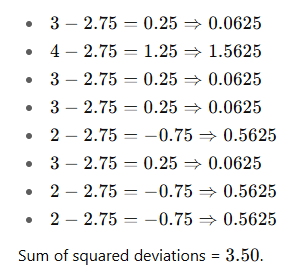
d = [3, 4, 3, 3, 2, 3, 2, 2]

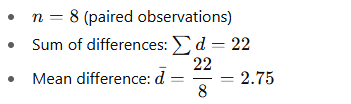
Now compute the sample standard deviation of the differences sd

Deviations from mean and squared deviations:

Sample variance of differences:

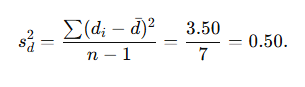
Sample standard deviation:

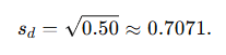
Standard error of the mean difference:

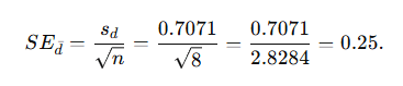
Step 3 — Compute the t statistic

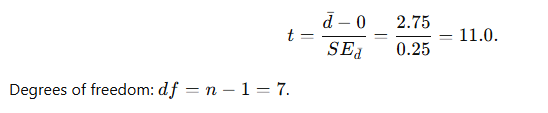
Step 4 — Decision (compare with critical value)

Since computed t=11.0t = 11.0t=11.0 is much larger than 2.365, we reject H₀ .

Conclusion: There is strong statistical evidence that the training program changed the athletes’ scores (here, the mean score increased by 2.75 units). The result is highly significant (p ≪ 0.01).

Step 5 — Effect size (optional but useful)

which is an extremely large effect — indicating a large practical change as well as statistical significance.

Assumptions reminder

Paired t-test assumes:

The differences did_idi are a random sample and observations are paired/related.
The distribution of differences is approximately normal (for small nnn). With n=8n=8n=8 it’s good to check a histogram or normality test; with larger nnn the t-test is robust.

Short interpretation

In this example the average improvement after training was 2.75 units (SD of differences = 0.71). The paired t-test yields t(7)=11.00, p<0.001. We therefore reject the null hypothesis and conclude the training produced a statistically significant improvement — also a very large practical effect (Cohen’s d ≈ 3.9d).

The Z-Test

The Z-test is the older, more straightforward test. It’s used when you have a clear, stable understanding of the “noise” in the entire population.

When to Use a Z-test:

Your sample size is large (typically n > 30).
You know the population standard deviation (σ).
Your data is (approximately) normally distributed.

The Z-Test Statistic Formula:
The formula varies slightly depending on what you’re comparing.

One-Sample Z-test (Comparing a sample mean to a population mean):
Z = (x̄ - μ) / (σ / √n)
- x̄: Your sample mean
- μ: The known population mean
- σ: The known population standard deviation
- n: Your sample size

Solved Example: The Soda Bottling Plant

A soda bottling plant claims its bottles are filled with 500 ml of liquid. The population standard deviation is known from the machinery specs to be 2 ml. A quality inspector takes a random sample of 35 bottles and finds an average fill of 499.2 ml. Test if the machine is under-filling at a significance level of 0.05.

Step 1: State the Hypotheses

Null Hypothesis (H₀): The machine is not under-filling. μ = 500 ml.
Alternative Hypothesis (H₁): The machine is under-filling. μ < 500 ml. (This is a one-tailed test)

Step 2: Calculate the Z-Test Statistic
We have:

x̄ = 499.2 ml
μ = 500 ml
σ = 2 ml
n = 35

Z = (499.2 - 500) / (2 / √35) = (-0.8) / (2 / 5.916) = (-0.8) / 0.338 ≈ -2.366

Step 3: Find the Critical Value and Make a Decision
For a one-tailed test at α = 0.05, the critical Z-value from the table is -1.645.

Decision Rule: If our Z-statistic is less than the critical value, we reject the null hypothesis.

Our Z (-2.366) < Critical Z (-1.645)

Step 4: Conclusion
We reject the null hypothesis. There is sufficient evidence at the 0.05 significance level to conclude that the machine is under-filling the bottles.

📊 Decision Rules Summary

Test	Condition	Decision Rule
Z-Test	σ known, n ≥ 30	Reject H₀ if
t-Test	σ unknown, n < 30	Reject H₀ if

Pro Tip: When your sample size is very large (n > 100), the t-distribution becomes almost identical to the normal Z-distribution. So, for large samples, even if you don’t know σ, you can often use a Z-test as a close approximation. However, statistical software will almost always use a t-test by default when σ is unknown.

🧠 Interpretation Tips

A large |t| or |Z| value → stronger evidence against H₀.
Always check p-values (probability of observing results if H₀ true).
Smaller p-value (< 0.05) → significant difference.
Report results as: “The mean yield was significantly higher for Fertilizer B (t(20)=2.07, p<0.05).”

Summary: Your Decision Flowchart

Start by asking: What am I comparing?
- One sample mean to a population mean? -> Use a one-sample test.
- Two independent group means? -> Use an independent two-sample test.
- The same group at two different times? -> Use a paired sample test.
For any of these, ask: Do I know the population standard deviation (σ)?
- YES -> Use a Z-test.
- NO -> Use a t-test. (This will be the case 99% of the time).

By understanding the “why” behind these tests, you can confidently choose the right tool to determine if the differences you see are real or just a trick of the light. Now go forth and test your hypotheses

🧮 Tools for Performing Tests

Excel: =T.TEST(range1, range2, tails, type)
Python: scipy.stats.ttest_ind() or ttest_rel()
R: t.test()
SPSS / Minitab / RStudio – user-friendly for non-coders

📚 Further Reading

Statistics for Business and Economics – Paul Newbold
Khan Academy: Hypothesis Testing
Towards Data Science: t-tests Explained
Practical Statistics for Data Scientists – Peter Bruce & Andrew Bruce

📈 Understanding t-Test and Z-Test: Comparing Means in Statistics

🌟 Introduction

🎯 What Are Hypothesis Tests?

⚖️ Difference Between t-Test and Z-Test