

Learn the different types of probability distributions, including Bernoulli, Binomial, Poisson, Normal, Exponential, Gamma, Beta, Weibull, t, Chi-Square and F distributions with formulas and examples.
Introduction
Probability distributions are one of the fundamental building blocks of statistics, data analytics, machine learning and decision-making.
Whenever we analyze data, we are often interested in questions such as:
- How likely is a particular outcome?
- What values can a variable take?
- How frequently do different outcomes occur?
- What is the probability of an event occurring within a particular interval?
- How much variation can we expect in the data?
- Does the observed data follow a particular statistical pattern?
Probability distributions provide a mathematical framework for answering these questions.
For example:
- The number of customers arriving at a store in one hour can be modeled using a Poisson distribution.
- The number of successful sales calls out of 20 calls can be modeled using a Binomial distribution.
- The height of individuals in a large population may be approximately modeled using a Normal distribution.
- The waiting time until the next customer arrives may be modeled using an Exponential distribution.
- The proportion of customers who respond to a campaign can be modeled using a Beta distribution.
- Product lifetime and failure-time data can often be modeled using Weibull or Lognormal distributions.
Understanding probability distributions is therefore essential for choosing appropriate statistical methods, estimating probabilities, conducting hypothesis tests, building predictive models and interpreting uncertainty.
This article introduces the major types of probability distributions and explains their characteristics, formulas, examples and applications.
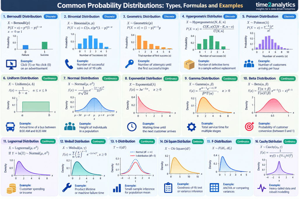
1. What is a Probability Distribution?
A probability distribution describes how the possible values of a random variable are distributed along with their associated probabilities.
A random variable is a variable whose value is determined by the outcome of a random process.
For example:
- Number of customers entering a store
- Number of defective products
- Daily rainfall
- Waiting time for a customer
- Monthly sales
- Temperature
- Number of clicks on an advertisement
A probability distribution tells us how likely different values of such a variable are.
For a valid probability distribution:
- Probabilities must be between 0 and 1.
- The probabilities of all possible outcomes must sum to 1 for a discrete random variable.
- For a continuous random variable, the total area under the probability density curve must equal 1.
NIST’s statistical handbook provides a comprehensive gallery of commonly used continuous and discrete probability distributions, while OpenStax introduces probability distributions as models used to represent uncertainty and calculate probabilities.
2. Two Major Types of Probability Distributions
Probability distributions can broadly be classified into:
1. Discrete probability distributions
Used when a random variable takes countable values, usually integers.
Examples:
- 0, 1, 2, 3, …
- Number of defective products
- Number of customers
- Number of successful transactions
2. Continuous probability distributions
Used when a random variable can take any value within an interval.
Examples:
- Height
- Weight
- Temperature
- Time
- Revenue
- Distance
The distinction is important because discrete distributions use a probability mass function (PMF), while continuous distributions are generally described using a probability density function (PDF).
3. Discrete Probability Distributions
3.1. Bernoulli Distribution
The Bernoulli distribution is the simplest discrete probability distribution.
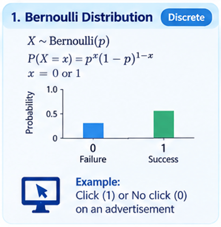
It represents an experiment with only two possible outcomes:
- Success
- Failure
Let:
- p = probability of success
- 1 − p = probability of failure
Then:
X ~ Bernoulli(p)
The probability function is:
P(X = x) = p^x × (1 − p)^(1 − x)
where:
x = 0 or 1
Example
Suppose an online advertisement has a 5% probability of generating a click.
For one impression:
- Click = 1
- No click = 0
- p = 0.05
Therefore, the click outcome can be represented using a Bernoulli distribution.
Applications
Bernoulli distributions are commonly used for:
- Yes/No responses
- Success/failure experiments
- Click/no-click events
- Purchase/no-purchase outcomes
- Defective/non-defective products
- Disease/no-disease classification
The Bernoulli distribution forms the foundation for several other discrete distributions, particularly the Binomial distribution.
3.2. Binomial Distribution
The Binomial distribution models the number of successes in a fixed number of independent Bernoulli trials when the probability of success remains constant.
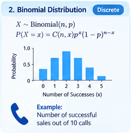
A Binomial experiment generally requires:
- A fixed number of trials, n.
- Two possible outcomes for each trial.
- Independence between trials.
- A constant probability of success, p.
The notation is:
X ~ Binomial(n, p)
Formula
P(X = x) = C(n, x) × p^x × (1 − p)^(n − x)
where:
- n = number of trials
- x = number of successes
- p = probability of success
- C(n, x) = number of combinations
Example
Suppose a salesperson makes 10 independent sales calls and the probability of obtaining a sale from each call is 20%.
What is the probability of obtaining exactly 3 sales?
Here:
- n = 10
- p = 0.20
- x = 3
Therefore:
P(X = 3) = C(10,3) × (0.20)^3 × (0.80)^7
This can be calculated using a statistical calculator or software.
Mean
Mean = n × p
Variance
Variance = n × p × (1 − p)
Applications
Binomial distribution is useful for:
- Number of successful sales
- Number of customers responding to a campaign
- Number of defective products in a sample
- Number of successful loan applications
- Number of patients responding to treatment
- Number of correct answers in a multiple-choice test
NIST identifies Binomial as one of the major discrete probability distributions, while OpenStax specifies the fixed-trial, two-outcome and independence conditions.
3.3. Geometric Distribution
The Geometric distribution models the number of independent trials required to obtain the first success.
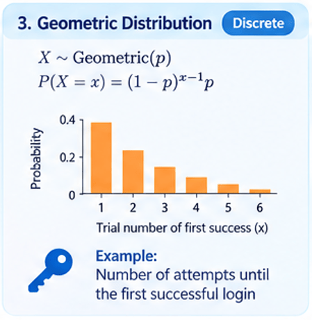
Formula
If X represents the trial on which the first success occurs:
P(X = x) = (1 − p)^(x − 1) × p
where:
- p = probability of success
- x = trial number of the first success
Example
Suppose the probability that a customer responds to an email campaign is 10%.
What is the probability that the first response occurs on the fourth email?
Here:
p = 0.10
x = 4
Therefore:
P(X = 4) = (0.90)^3 × 0.10
Applications
Geometric distributions can be used for:
- Number of calls until the first sale
- Number of attempts until a successful login
- Number of trials until a successful experiment
- Number of customers contacted until the first conversion
OpenStax defines the geometric distribution as the distribution of the number of independent trials until the first success.
3.4. Hypergeometric Distribution
The Hypergeometric distribution is used when sampling is conducted without replacement.
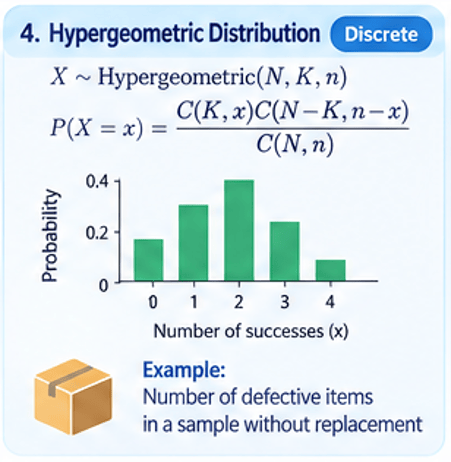
This is an important difference between the Hypergeometric and Binomial distributions.
Example
Suppose a warehouse contains:
- 100 products
- 10 defective products
- 90 good products
A quality inspector randomly selects 5 products without replacement.
The Hypergeometric distribution can be used to determine the probability of selecting exactly 2 defective products.
Formula
P(X = x) = [C(K,x) × C(N−K,n−x)] ÷ C(N,n)
where:
- N = population size
- K = number of successes in the population
- n = sample size
- x = observed number of successes
Applications
It is useful for:
- Quality control
- Sampling inspection
- Auditing
- Card and lottery problems
- Finite population sampling
The key distinction is:
Binomial → independent trials with a constant probability.
Hypergeometric → sampling without replacement from a finite population.
OpenStax specifically highlights the without-replacement distinction between Hypergeometric and Binomial experiments.
3.5. Poisson Distribution
The Poisson distribution models the number of times an event occurs within a specified interval of time, space or another measurement.
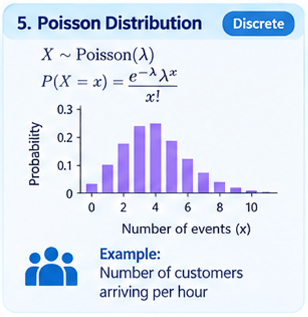
Examples include:
- Number of customers arriving per minute
- Number of website errors per hour
- Number of calls received by a call centre
- Number of accidents per month
- Number of defects per metre of material
The notation is:
X ~ Poisson(λ)
where λ represents the average number of occurrences in the specified interval.
Formula
P(X = x) = (e^(−λ) × λ^x) ÷ x!
Example
Suppose a call centre receives an average of 8 calls per minute.
Then:
λ = 8
The Poisson distribution can be used to estimate the probability of receiving exactly 5 calls in a particular minute.
Mean
Mean = λ
Variance
Variance = λ
This equality between the mean and variance is one of the defining characteristics of the Poisson distribution.
Applications
Poisson distribution is widely used in:
- Queueing analysis
- Call centres
- Website traffic
- Insurance claims
- Accident analysis
- Manufacturing defects
- Hospital arrivals
- Network failures
NIST defines the Poisson distribution as a model for the number of events occurring within a given interval, while OpenStax provides the same interpretation for event counts over time or space.
4. Continuous Probability Distributions
Continuous random variables can take any value within a range.
For example, the weight of a person might be:
65 kg, 65.1 kg, 65.15 kg, 65.153 kg, …
There are theoretically infinitely many possible values.
For continuous distributions, probability is represented by the area under the probability density curve.
An important property is:
P(X = a) = 0
for any exact single value a in a continuous distribution.
Instead, we calculate probabilities over intervals, such as:
P(60 < X < 70)
OpenStax describes continuous random variables as variables that can take values across an interval and introduces the Uniform, Exponential and Normal distributions as important continuous distributions.
4.1. Uniform Distribution
The Uniform distribution assumes that all values within a specified interval have equal density.
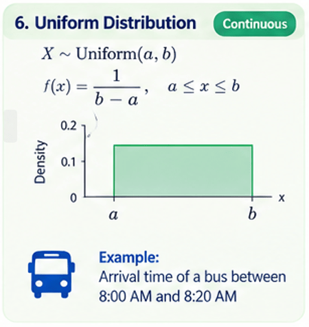
The notation is:
X ~ Uniform(a,b)
Formula
For a ≤ x ≤ b:
f(x) = 1 ÷ (b − a)
Example
Suppose a bus arrives randomly between 8:00 AM and 8:20 AM.
If every arrival time within this interval is considered equally likely, the waiting time can be modeled using a Uniform distribution.
If the waiting time is represented in minutes:
X ~ Uniform(0,20)
The probability that the bus arrives within the first 5 minutes is:
P(0 ≤ X ≤ 5) = 5 ÷ 20 = 0.25
Therefore, the probability is 25%.
Applications
Uniform distribution is useful for:
- Random number generation
- Simulation
- Random arrival assumptions
- Sampling
- Certain scheduling models
4.2. Normal Distribution
The Normal distribution is one of the most important probability distributions in statistics.
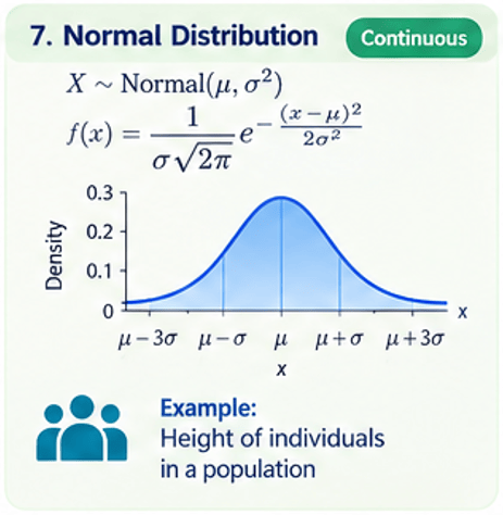
It is commonly called the bell-shaped distribution or Gaussian distribution.
The notation is:
X ~ Normal(μ, σ²)
where:
- μ = mean
- σ = standard deviation
- σ² = variance
Probability Density Function
f(x) = [1 ÷ (σ × √(2π))] × e^[−(x − μ)² ÷ (2σ²)]
Characteristics
A Normal distribution is:
- Symmetric
- Bell-shaped
- Unimodal
- Centered around the mean
- Characterized by its mean and standard deviation
For a perfectly Normal distribution:
Mean = Median = Mode
NIST describes the Normal distribution as symmetric and unimodal, with mean and standard deviation determining its location and scale.
4.3. The 68–95–99.7 Rule
For a Normal distribution:
Approximately:
- 68% of observations fall within ±1 standard deviation of the mean.
- 95% fall within ±2 standard deviations.
- 99.7% fall within ±3 standard deviations.
Example
Suppose examination scores are approximately Normally distributed with:
- Mean = 70
- Standard deviation = 10
Approximately 68% of students would be expected to score between:
70 − 10 = 60
and
70 + 10 = 80
Therefore, approximately 68% of observations lie between 60 and 80.
4.4 Standard Normal Distribution
A Standard Normal distribution has:
Mean = 0
Standard deviation = 1
A raw observation can be converted to a standard score using the z-score.
Formula
z = (x − μ) ÷ σ
Example
Suppose:
- Mean = 70
- Standard deviation = 10
- Student score = 85
Then:
z = (85 − 70) ÷ 10
z = 1.5
The student’s score is therefore 1.5 standard deviations above the mean.
4.5. Exponential Distribution
The Exponential distribution is commonly used to model waiting times between events when events occur continuously at a constant average rate.
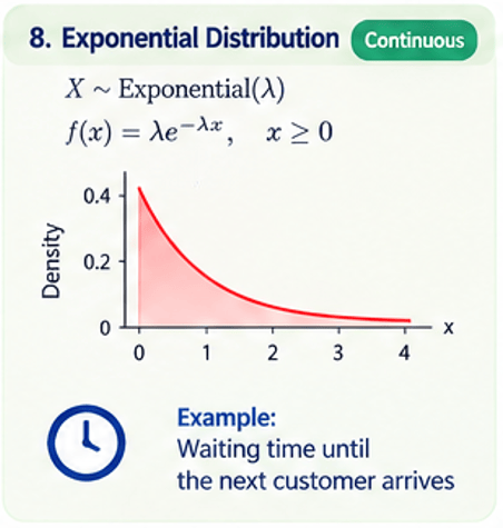
The notation is:
X ~ Exponential(λ)
where λ represents the event rate.
Formula
For x ≥ 0:
f(x) = λ × e^(−λx)
Example
Suppose customers arrive at a service counter at an average rate of 6 customers per hour.
Then:
λ = 6 per hour
The Exponential distribution can be used to model the waiting time until the next customer arrives under the relevant assumptions.
Applications
- Waiting time
- Customer arrivals
- Equipment failure
- Service systems
- Reliability analysis
- Queueing systems
The Exponential distribution is also a special case of the Gamma distribution.
4.6. Gamma Distribution
The Gamma distribution is a flexible continuous distribution for modeling positive-valued variables, particularly waiting times and accumulated event times.
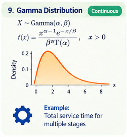
A common parameterization uses:
- α = shape parameter
- β = scale parameter
Formula
f(x) = x^(α−1) × e^(−x/β) ÷ [β^α × Γ(α)]
for:
x > 0
where Γ(α) is the Gamma function.
Example
Suppose a service system requires several independent service stages, and we are interested in the total time required for those stages.
The Gamma distribution can provide a useful model for the accumulated waiting or service time under suitable assumptions.
Applications
- Waiting times
- Reliability analysis
- Insurance
- Rainfall amounts
- Service times
- Bayesian statistics
NIST notes that the Gamma distribution has different common parameterizations, so analysts should always check whether a source uses shape-scale or shape-rate parameters.
This is an important practical point because the same symbols may represent different parameters in different statistical software packages.
4.7. Beta Distribution
The Beta distribution is particularly useful for modeling variables that are constrained to the interval 0 to 1.
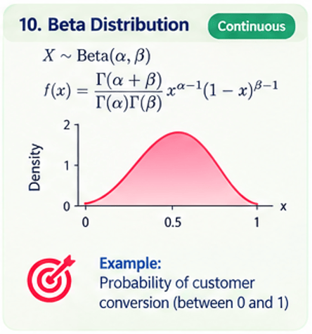
The notation is:
X ~ Beta(α, β)
where α and β are shape parameters.
Formula
f(x) = [Γ(α + β) ÷ (Γ(α)Γ(β))] × x^(α−1) × (1−x)^(β−1)
for:
0 < x < 1
Example
Suppose a digital marketing analyst is estimating the probability that a visitor converts.
The conversion probability must lie between:
0 and 1
or equivalently:
0% and 100%
A Beta distribution can therefore be used as a model for an uncertain conversion probability.
Applications
- Conversion probabilities
- Click-through probabilities
- Proportions
- Bayesian analysis
- A/B testing
- Success probabilities
The Beta distribution is especially important in Bayesian statistics because it is a conjugate prior for the Binomial probability parameter under the standard Beta-Binomial model. SciPy and NIST both document the Beta distribution and its shape-parameter representation.
4.8. Lognormal Distribution
A variable is Lognormally distributed when its logarithm follows a Normal distribution.
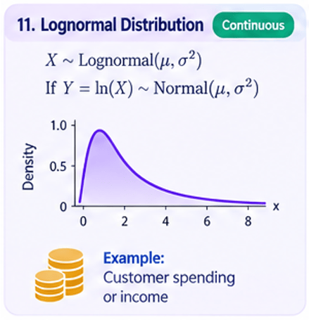
If:
Y = ln(X)
and Y follows a Normal distribution, then X follows a Lognormal distribution.
Example
Suppose customer spending is strongly right-skewed:
- Most customers spend relatively small amounts.
- A smaller number spend substantially more.
A Lognormal distribution may be a useful candidate model because it naturally represents positive, right-skewed values.
Applications
- Income
- Customer spending
- Financial variables
- Product lifetimes
- Environmental measurements
- Particle sizes
NIST includes Lognormal among its commonly used continuous distributions and discusses it extensively in reliability applications.
4.9. Weibull Distribution
The Weibull distribution is widely used in reliability engineering and survival analysis.
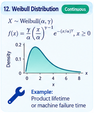
It is particularly useful because its shape parameter allows the distribution to represent different types of failure behavior.
A common two-parameter Weibull model uses:
- α = scale parameter
- γ = shape parameter
Formula
A common form of the PDF is:
f(x) = (γ/α) × (x/α)^(γ−1) × e^[−(x/α)^γ]
for:
x ≥ 0
Why is Weibull important?
The shape parameter can describe different failure patterns.
If:
γ < 1
the failure rate tends to decrease.
If:
γ = 1
the Weibull distribution reduces to the Exponential distribution.
If:
γ > 1
the failure rate tends to increase.
Applications
- Machine failure
- Equipment reliability
- Product lifetime
- Survival analysis
- Maintenance planning
- Engineering reliability
NIST identifies Weibull as an important lifetime and reliability distribution and provides its PDF and parameterization.
4.10. Student’s t-Distribution
The Student’s t-distribution is particularly important when estimating or testing a population mean when the population standard deviation is unknown, especially for smaller samples under appropriate assumptions.
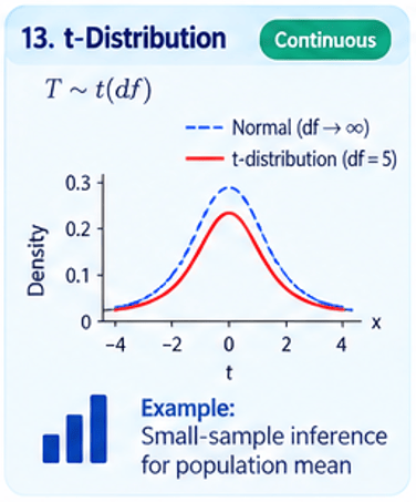
It is symmetric around zero and has heavier tails than the Standard Normal distribution.
The distribution is characterized by its:
degrees of freedom (df)
As the degrees of freedom increase, the t-distribution approaches the Standard Normal distribution.
Example
Suppose a researcher has a sample of 15 observations and wants to test whether the population mean differs from a hypothesized value.
If the population standard deviation is unknown and the assumptions for the t-test are reasonable, the t-distribution is used.
Applications
- One-sample t-test
- Two-sample t-test
- Confidence intervals for means
- Regression coefficient inference
NIST includes the t-distribution among its major probability distributions and provides critical-value tables for it.
4.11. Chi-Square Distribution
The Chi-Square distribution is widely used in statistical inference.
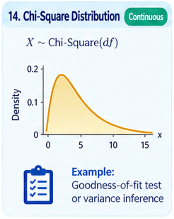
If independent Standard Normal random variables are squared and summed, the resulting variable follows a Chi-Square distribution with degrees of freedom equal to the number of squared Standard Normal variables.
Key characteristic
The Chi-Square distribution:
- Is non-negative.
- Is right-skewed, particularly with small degrees of freedom.
- Changes shape as degrees of freedom increase.
Applications
It is commonly used in:
- Chi-square tests of independence
- Goodness-of-fit tests
- Tests involving population variance
- Confidence intervals for variance
- Statistical inference
NIST provides critical-value tables and distribution information for the Chi-Square distribution.
4.12. F-Distribution
The F-distribution is especially important when comparing variances and in analysis of variance (ANOVA).
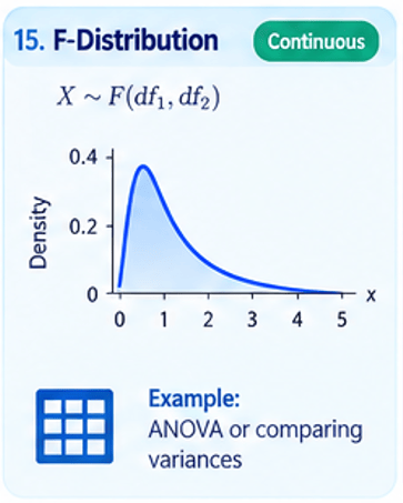
Conceptually, an F-statistic is a ratio of two variance estimates.
In one-way ANOVA:
F = MS_Between ÷ MS_Within
where:
- MS_Between = Mean Square Between Groups
- MS_Within = Mean Square Within Groups
Example
Suppose a researcher compares the average sales generated by four different advertising strategies.
ANOVA evaluates whether the variation between the group means is large relative to the variation within the groups.
A large F-statistic can provide evidence against the null hypothesis, but the final statistical decision should be based on the p-value or comparison with the appropriate critical F-value, considering the relevant degrees of freedom.
Applications
- ANOVA
- Comparing variances
- Regression significance testing
- Variance-ratio tests
NIST lists the F-distribution as one of the major continuous distributions and provides critical-value tables for different numerator and denominator degrees of freedom.
4.13. Cauchy Distribution
The Cauchy distribution is a continuous distribution with very heavy tails.
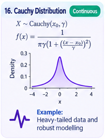
It is important because its mean and variance do not exist in the conventional finite sense.
This makes it a useful example of why statistical methods that depend on finite means or variances cannot automatically be applied to every distribution.
Applications
Cauchy distributions arise in:
- Certain physical measurement models
- Robust statistical modelling
- Ratio-related phenomena
- Theoretical statistics
NIST includes the Cauchy distribution in its gallery of commonly studied continuous distributions.
5. A Comparison of Important Probability Distributions
| Distribution | Type | Typical Variable | Key Parameter(s) | Example |
|---|---|---|---|---|
| Bernoulli | Discrete | Binary outcome | p | Click / No click |
| Binomial | Discrete | Number of successes | n, p | Sales from 20 calls |
| Geometric | Discrete | Trials until first success | p | Calls until first sale |
| Hypergeometric | Discrete | Successes in sample without replacement | N, K, n | Defective items in inspection |
| Poisson | Discrete | Number of events | λ | Customers per minute |
| Uniform | Continuous | Value within an interval | a, b | Random arrival time |
| Normal | Continuous | Symmetric measurement | μ, σ | Height or test scores |
| Exponential | Continuous | Waiting time | λ | Time until next arrival |
| Gamma | Continuous | Positive waiting/accumulation time | α, β | Total service time |
| Beta | Continuous | Proportion/probability | α, β | Conversion probability |
| Lognormal | Continuous | Positive right-skewed variable | μ, σ of log(X) | Customer spending |
| Weibull | Continuous | Lifetime/failure time | Shape, scale | Machine lifetime |
| t | Continuous | Standardized mean-related statistic | df | Small-sample inference |
| Chi-Square | Continuous | Variance-related statistic | df | Goodness-of-fit |
| F | Continuous | Ratio of variance estimates | df₁, df₂ | ANOVA |
| Cauchy | Continuous | Heavy-tailed variable | Location, scale | Robust/theoretical modelling |
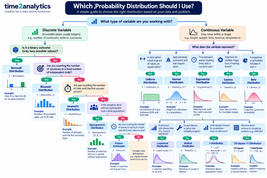
6. How Do You Choose the Right Distribution?
Choosing a probability distribution should not be based simply on which distribution is most familiar.
The analyst should consider:
Step 1: What type of variable is being analyzed?
Is it:
- Binary?
- A count?
- A proportion?
- A continuous measurement?
- A waiting time?
- A lifetime?
- A positive monetary value?
Step 2: What values can the variable take?
For example:
Binary: 0 or 1
Count: 0, 1, 2, 3, …
Proportion: 0 to 1
Time: Usually non-negative
Normal measurement: Potentially any real number
Step 3: What does the data look like?
Examine:
- Histogram
- Density plot
- Box plot
- Q-Q plot
- Skewness
- Kurtosis
- Outliers
Step 4: What assumptions are appropriate?
For example:
Binomial: fixed number of independent trials and constant success probability.
Poisson: event-count setting with an appropriate rate assumption.
Normal: symmetric continuous data or situations where Normal modelling is justified.
Exponential: waiting-time setting under an appropriate constant-rate/memoryless model.
Step 5: Assess model fit
Possible tools include:
- Q-Q plots
- Probability plots
- Goodness-of-fit tests
- AIC/BIC
- Kolmogorov-Smirnov test
- Anderson-Darling test
- Chi-square goodness-of-fit test
Statistical software such as Python’s scipy.stats provides a wide range of discrete and continuous distributions along with goodness-of-fit and statistical testing functionality.
7. Distribution Selection: Practical Examples
Example 1: Online Advertising
Suppose an organization wants to model whether a user clicks an advertisement.
Possible distribution:
Bernoulli
because the outcome is:
Click = 1
No click = 0
If we instead examine the number of clicks among 10,000 independent impressions with a constant probability of click, a Binomial model may be appropriate under its assumptions.
Example 2: Call Centre
Suppose a call centre receives an average of 20 calls every hour.
The number of calls received in an hour can potentially be modeled using:
Poisson distribution
If the question changes to:
“How long will we wait until the next call?”
then an:
Exponential distribution
may be appropriate under the corresponding rate assumptions.
This illustrates an important relationship:
Poisson → number of events
Exponential → waiting time between events
8. Distribution Relationships
Many probability distributions are mathematically related.
Some important relationships include:
Bernoulli → Binomial
A Binomial variable can be viewed as the sum of independent Bernoulli trials.
Binomial → Poisson
Under appropriate conditions, a Binomial distribution with a large number of trials and small success probability can be approximated by a Poisson distribution.
Poisson → Exponential
A Poisson process describes event counts, while the corresponding Exponential distribution describes waiting times between events under the homogeneous Poisson-process assumptions.
Gamma → Exponential
The Exponential distribution is a special case of the Gamma distribution.
Normal → Chi-Square
The sum of squares of independent Standard Normal variables produces a Chi-Square distribution.
Normal → t
The t-distribution arises from a standardized Normal variable combined with an independent Chi-Square-based variance estimate.
Chi-Square → F
The F-distribution can be constructed from ratios of independent Chi-Square variables after scaling by their respective degrees of freedom.
Understanding these relationships helps analysts see probability distributions not as isolated formulas but as an interconnected statistical system.
NIST’s distribution gallery explicitly organizes many of these commonly used distributions and their relationships.
9. Probability Distributions in Data Analytics
Probability distributions play an important role throughout the analytics lifecycle.
Descriptive Analytics
Distributions help analysts understand:
- Central tendency
- Variability
- Skewness
- Outliers
- Data shape
Predictive Analytics
Distributions help quantify:
- Future uncertainty
- Event probabilities
- Customer behaviour
- Failure probabilities
- Demand
Inferential Statistics
Distributions provide the foundation for:
- Confidence intervals
- Hypothesis tests
- ANOVA
- Regression inference
- Sampling distributions
Machine Learning
Distributional assumptions can be important in:
- Probabilistic models
- Bayesian modelling
- Generative models
- Classification
- Forecasting
- Risk modelling
Decision Analytics
Probability distributions allow organizations to evaluate uncertainty in:
- Demand
- Revenue
- Risk
- Inventory
- Customer arrivals
- Project completion
- Equipment failure
10. Probability Distribution vs Sampling Distribution
These two concepts are often confused.
Probability Distribution
Describes the possible values of a random variable.
Example:
Distribution of individual customer purchase amounts.
Sampling Distribution
Describes the distribution of a statistic calculated from repeated samples.
Example:
Distribution of sample means obtained from many samples.
Sampling distributions are fundamental to inferential statistics and help explain why statistics such as the sample mean, t-statistic, Chi-Square statistic and F-statistic have particular probability distributions.
11. Why Distribution Matters in Statistical Analysis
Choosing an inappropriate distribution can lead to:
- Incorrect probability estimates
- Misleading confidence intervals
- Invalid hypothesis tests
- Poor predictions
- Incorrect risk estimates
- Wrong business decisions
For example, suppose a variable is highly right-skewed and positive, but the analyst automatically assumes a Normal distribution.
The model may predict negative values even though the variable cannot logically be negative.
Similarly, treating a count variable as continuous without considering its distribution may result in an inappropriate statistical model.
Therefore:
Distribution selection is not merely a mathematical exercise; it is a model-selection decision.
12. Common Mistakes When Using Probability Distributions
Mistake 1: Assuming everything is Normal
Not every dataset follows a Normal distribution.
Mistake 2: Confusing discrete and continuous variables
The number of customers is discrete, while customer waiting time is generally continuous.
Mistake 3: Ignoring the sampling mechanism
Sampling with replacement and without replacement can lead to different probability models.
Mistake 4: Ignoring skewness
Positive variables such as income, spending and some waiting times can be strongly right-skewed.
Mistake 5: Ignoring parameterization
Gamma, Weibull and other distributions can be parameterized differently by different textbooks and software packages.
Mistake 6: Choosing a distribution only because it fits visually
Visual fit is useful, but analysts should also consider the data-generating process, assumptions and statistical diagnostics.
13. Probability Distributions and Python
Python provides extensive support for probability distributions through libraries such as SciPy.
For example, scipy.stats includes:
bernoullibinomgeomhypergeompoissonuniformnormexpongammabetaweibulllognormtchisquaref
SciPy also provides functions for probability calculations, random-number generation, distribution fitting and statistical tests.
For example, the following Python code can calculate the probability of exactly 3 successes in a Binomial experiment:
from scipy.stats import binomprobability = binom.pmf(3, n=10, p=0.20)print(probability)
Similarly, the probability associated with a Normal distribution can be calculated using:
from scipy.stats import normprobability = norm.cdf(85, loc=70, scale=10)print(probability)
This makes probability distributions highly practical for modern data analytics.
14. A Simple Distribution Selection Guide
| If your variable represents… | Consider… |
|---|---|
| Yes/No outcome | Bernoulli |
| Number of successes in fixed trials | Binomial |
| Trials until first success | Geometric |
| Sample successes without replacement | Hypergeometric |
| Number of events in an interval | Poisson |
| Value equally likely within a range | Uniform |
| Approximately symmetric continuous measurement | Normal |
| Waiting time until next event | Exponential |
| Accumulated waiting/service time | Gamma |
| Probability or proportion between 0 and 1 | Beta |
| Positive right-skewed measurement | Lognormal |
| Failure/lifetime data | Weibull |
| Small-sample mean inference | t |
| Variance/goodness-of-fit inference | Chi-Square |
| Ratio of variance estimates / ANOVA | F |
| Extremely heavy-tailed data | Cauchy |
This table should be treated as a starting point rather than an automatic distribution-selection rule. The underlying data-generating process and empirical evidence should guide the final model choice.
15. Key Takeaways
Probability distributions provide a framework for understanding uncertainty.
The most important distributions to remember include:
Discrete
Bernoulli → Binomial → Geometric → Hypergeometric → Poisson
Continuous
Uniform → Normal → Exponential → Gamma → Beta → Lognormal → Weibull
Statistical inference
t → Chi-Square → F
Each distribution answers a different type of probability question.
The central lesson is:
Choose the distribution based on the nature of the random variable, the data-generating process, and the assumptions—not simply because a distribution is popular.
For data analysts, understanding distributions provides the foundation for moving from descriptive statistics to probability, inference, prediction and decision-making.
Conclusion
Probability distributions are at the heart of statistics and analytics.
From the simple Bernoulli distribution representing a binary outcome to the Normal distribution used extensively in statistical modelling, and from the Poisson distribution used to model event counts to the Weibull distribution used in reliability analysis, each distribution provides a different way of representing uncertainty.
The most important skill is not memorizing every probability density function.
Instead, analysts should learn to ask:
What type of variable am I analyzing?
What values can it take?
How was the data generated?
What does the empirical distribution look like?
Which probability distribution provides a reasonable representation of that process?
Once these questions are answered, probability distributions become much more than statistical formulas. They become practical tools for forecasting, risk assessment, hypothesis testing, predictive modelling and data-driven decision-making.
Quick Reference: Important Formulas
For convenient reference, the principal formulas discussed in this article are summarized below.
| Distribution | Probability / Density Formula |
|---|---|
| Bernoulli | P(X=x) = p^x × (1−p)^(1−x) |
| Binomial | P(X=x) = C(n,x) × p^x × (1−p)^(n−x) |
| Geometric | P(X=x) = (1−p)^(x−1) × p |
| Hypergeometric | P(X=x) = [C(K,x) × C(N−K,n−x)] ÷ C(N,n) |
| Poisson | P(X=x) = (e^(−λ) × λ^x) ÷ x! |
| Uniform | f(x) = 1 ÷ (b−a) |
| Normal | f(x) = [1 ÷ (σ√(2π))] × e^[−(x−μ)² ÷ (2σ²)] |
| Exponential | f(x) = λ × e^(−λx) |
| Gamma | f(x) = x^(α−1)e^(−x/β) ÷ [β^αΓ(α)] |
| Beta | f(x) = [Γ(α+β) ÷ Γ(α)Γ(β)] × x^(α−1)(1−x)^(β−1) |
| Weibull | f(x) = (γ/α)(x/α)^(γ−1)e^[−(x/α)^γ] |
Note: Some distributions, particularly Gamma, Weibull and related families, have multiple parameterizations. Always verify the parameter definitions used by the textbook, statistical software or analytical package being used. NIST explicitly cautions that equivalent formulas may use different parameterizations.
References and Further Reading
- NIST/SEMATECH e-Handbook of Statistical Methods — Probability Distributions. The NIST handbook provides a detailed gallery of Normal, Uniform, Cauchy, t, F, Chi-Square, Exponential, Weibull, Lognormal, Gamma, Beta, Binomial and Poisson distributions.
NIST/SEMATECH e-Handbook of Statistical Methods - OpenStax — Introductory Statistics 2e. Provides accessible explanations and formulas for discrete and continuous probability distributions, including Binomial, Geometric, Hypergeometric, Poisson, Uniform, Exponential and Normal distributions.
OpenStax Introductory Statistics 2e - OpenStax — Principles of Data Science. Provides an applied perspective on probability distributions and their use in data science, including Python applications.
OpenStax Principles of Data Science - SciPy Documentation — scipy.stats. Provides implementations of a large collection of discrete and continuous probability distributions and statistical functions in Python.
SciPy Statistical Functions - Devore, J. L. Probability and Statistics for Engineering and the Sciences. Cengage Learning.
- Montgomery, D. C. & Runger, G. C. Applied Statistics and Probability for Engineers. Wiley.
- Casella, G. & Berger, R. L. Statistical Inference. Cengage Learning.








Leave a comment